
Level: ⚫⚫⚫⚪⚪ Advanced
Requirements
- Local copy of the MAgPIE model (https://github.com/magpiemodel/magpie)
- Have R installed (https://www.r-project.org/)
- (For validation.pdf creation:) Have Latex installed (e.g., MiKTeX https://miktex.org/howto/install-miktex)
- Have completed a MAgPIE run OR downloaded existing MAgPIE runs (https://zenodo.org/record/2572620#.X8Zr9RbPw2w or https://zenodo.org/record/5417474#.YeAf8_DMJaQ)
Content
- Use model-internal R-scripts for output analysis.
- Know where to find the automated validation PDF and how it is structured.
- Use the evaluation tool
appResultsLocalof the libraryshinyresults. - Use the
magpie4package for output analysis. - Analyse outputs with the
gdxpackage.
Overview
Introduction
After having successfully started and accomplished a simulation run, the
next step is to evaluate the simulation results. In case you have not
yet conducted an own MAgPIE simulation or your simulation is still
running, you can download model runs produced for Mishra et al. (2021)
(https://doi.org/10.5194/gmd-14-6467-2021).
These runs were created with version 4.3.5 of the MAgPIE model
(https://github.com/magpiemodel/magpie/tree/master).
You can download these runs as tgz folder from Zenodo (choose the folder
magpie_v4.3.5_gmd-2021-76.tgz at https://zenodo.org/record/5417474#.YeAf8_DMJaQ)
and copy the folders containing the simulation
results into the output folder of your local version of the MAgPIE
model (Note: if you freshly cloned the model and did not set up a run yet, you
will have to create an empty output folder first).
There are several ways to assess and evaluate MAgPIE results. This tutorial gives an overview on different tools and options that can be used to analyse model outputs.
For each simulation, results are written into a subfolder of the output folder.
This subfolder is created automatically. Its name is a combination of the
model title and date. This is defined in the default.cfg
(cfg$results_folder <- "output/:title::date:").
Model-internal R-scripts for output analysis
Manual execution of model-internal R-scripts
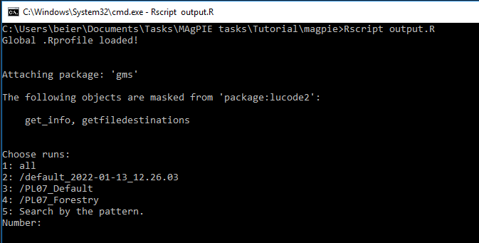
There are several output scripts that can be executed after the model run has finished. These R scripts can be found in the folder scripts/output. They can be selected and executed via the command window. To do so, windows users can open a command line prompt in the MAgPIE model folder by using shift + rightClick and then selecting open command window here option.
In the command prompt, use the following command:
Rscript output.R
You are now asked to choose the simulation run for which you would like to execute an output script.
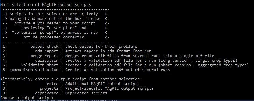
Next, you can choose which output scripts you want to execute:
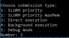
The last step is to select the run submission type, e.g. “Direct execution”:
Now, the selected script will be executed. After completion, the results are written in the respective folder of the simulation run inside the output folder of the model.
Model-internal R-script selection in the config file
In the file config/default.cfg, it is possible to specify which of these
output R scripts are executed after a model run is finished.
In the default MAgPIE configuration, the scripts output_check
rds_report (to be used in appResultsLocal; see below),
validation_short and extra/disaggregation are selected via cfg$output:
cfg$output <- c("output_check", "rds_report", "validation_short",
                "extra/disaggregation")
Automated model validation
The automated model validation is an example of output
analysis based on model-internal scripts (see
above).
If the validation script is executed (either by selection via cfg$output as
explained above or
by execution via the command window as explained
above,
a standard evaluation PDF is created that validates numerous
model outputs with a validation database containing historical data and
projections for most outputs returned by the model, either visually or
via statistical tests. A standard evaluation PDF consists of hundreds of
evaluation outputs and usually has a length of around 1800 pages. By
evaluating the model outputs on such a broad level rather than focusing
only on key outputs, it allows getting a more complete picture of the
corresponding simulation. As an example of such validation files, you
can download the evaluation documents produced for all runs shown in the
MAgPIE 4 framework paper (https://doi.org/10.5281/zenodo.1485303)
or run the “validation” or “validation_short” output scripts as explained above.
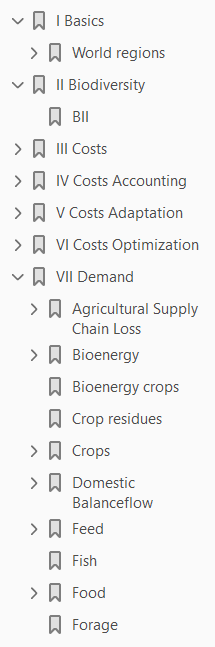
The table of contents of the validation PDF gives a good overview over the model outputs that can be simulated with a MAgPIE standard simulation, even though the validation PDF only shows a subset of possible model outputs:
Interactive scenario analysis
The automated model validation PDF is a good tool for visually evaluating a broad range of model outputs. However, comparison between model runs, i.e. between different scenarios, is rather difficult and inconvenient with the different model results being scattered across different large PDF files.
To overcome this issue, we developed the interactive scenario analysis
and evaluation tools appResultsLocal (and appResults for the use within
the PIK network) as part of the library shinyresults
(https://github.com/pik-piam/shinyresults). It facilitates the evaluation of
results with plots for multiple scenarios including historical data and other
projections based on an interactive selection of regions and variables.
You can use this tool by running the following R command in the main
folder of your model, which will automatically collect all runs in the
output folder and visualize them:
shinyresults::appResultsLocal()
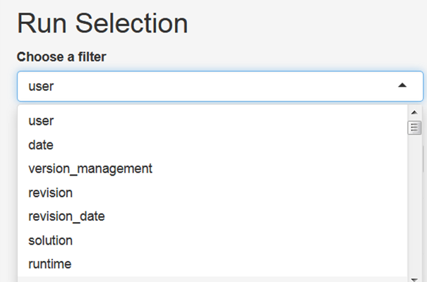
This command opens an interactive window, where you can select the simulations that you want to evaluate.
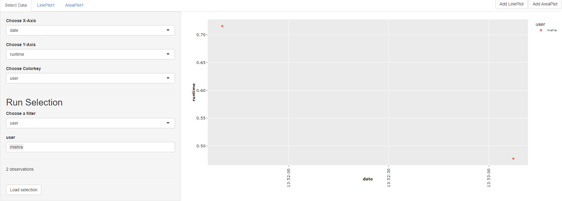
You can use filters to select a subset of all runs stored in the output folder of the model, for example by searching for runs that have been finished at a certain day, have been created by a certain user or by searching for keywords in the title of the simulation runs:
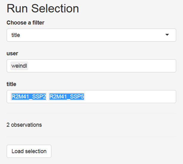
After having selected the subset of runs that you want to analyse, click the button Load selection. Now, you can click on the tab LinePLot. You will then see on the right hand side line plots showing the development of population for historical and future time steps for all model regions and on the global scale:
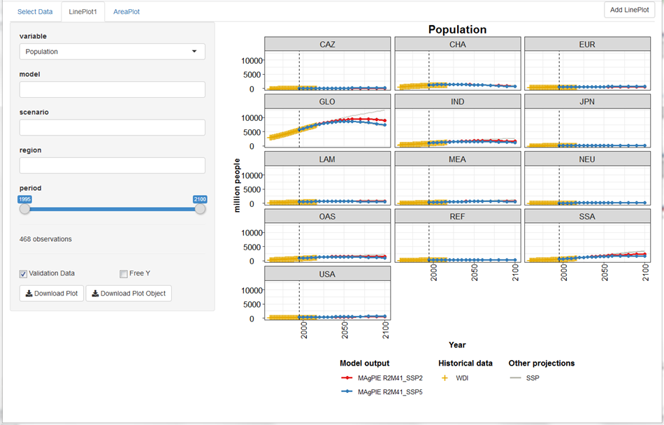
Now, choose a variable of your interest, either by scrolling through the drop-down menu or write a key word in the input field, e.g. “cropland”, to reduce the options in the menu.
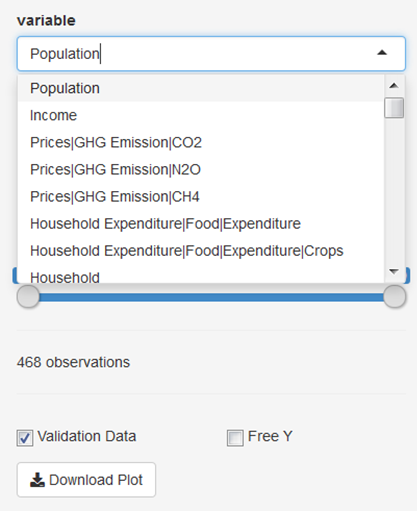
Make yourself familiar with the features of the app! You can, for example, select a subset of regions or a subset of time steps for which the results should be plotted. Moreover, you can free the y-axis, include or exclude validation data (if available) and download the plot.
Analysis of outputs with the magpie4 library
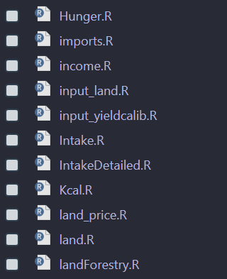
If you want to go beyond visual output analysis and predefined output evaluation facilitated by scripts, you can use the functionality of the R package magpie4 (https://github.com/pik-piam/magpie4). This library contains a list of functions for extracting outputs from the MAgPIE model, which are also the basis for the generation of the automated validation PDF. For a quick overview of the functions included in the library, you can have a look in the folder magpie4/R. The following figure shows a subset of R-files included in magpie4/R:
To make yourself familiar with this library, you can open an R/RStudio session and set the MAgPIE model folder as working directory. This can be done by using the following command:
setwd("/path/to/your/magpie/model/folder")
Then, load the library and call the help pages:
library(magpie4)
?magpie4
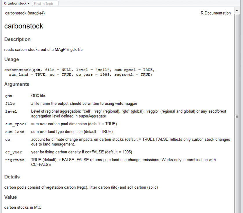
You can click on the index and search for interesting functions, e.g. carbonstock, and read the respective help page:
Analyzing outputs with the gdx library
The gdx2 library (https://github.com/pik-piam/gdx2) allows to
directly access objects contained in the fulldata.gdx file via the
function readGDX. A pragmatic way to learn how to use this function
for the extraction of interesting information from the fulldata.gdx is
to open R files of the magpie4 library within Rstudio. Most of the
magpie4 functions make use of readGDX.
In the function magpie4::carbonstock(), we see several
instances where gdx2::readGDX is used,
e.g.:
a <- readGDX(gdx, "ov_carbon_stock", select=list(type = "level"), react = "silent")
sm_cc_carbon <- readGDX(gdx, "sm_cc_carbon2", react = "silent")
ov_land <- readGDX(gdx, "ov_land", select = list(type = "level"))
fm_carbon_density <- readGDX(gdx, "fm_carbon_density")[,t,]
It is possible to extract various GAMS objects like “sets”,
“equations”, “parameters”, “variables” and “aliases” with
readGDX.
With the argument select = list(type = “level”), you can select the level values
of endogenous variables, with select = list(type = “marginal”) you can
extract the marginal values of these variables.
Exercises (click on the arrows to uncover the solution)
Open a validation pdf (either in a folder containing your own simulation results or the downloaded MAgPIE simulation runs and (a) make yourself familiar with the structure of the document and the hierarchy of outputs as displayed by the table of contents and; (b) have a look at some figures displaying model outputs of your interest.
Execute the model-internal output script `rds report` via the command window. This script collects the results of several report-functions - that calculate many key output variables like Production, Land Use or Yields - and writes them into an rds file.
- open a command window in the main MAgPIE model folder
- select model run by typing in the respective number and press
ENTER- select
rds reportby pressing2andENTER- select
Direct executionby pressing3andENTERStart the interactive scenario analysis tool using the shinyresults R library, select one particular model run using the title filter and look at a variable of your choice.
- Open an R session in the main folder structure of the MAgPIE model folder
- Execute the command
shinyresults::appResultsLocal()- After the interactive site has opened, select
titleas a filter in theSelect Datatab and look for the simulation run of your choice- Click on
Load selectionand open theLinePlot1orAreaPlot1tab- Select a variable of your choice and optionally also a particular scenario or region.
Find out how to include a custom validation file in the interactive scenario analysis tool. (This can be useful when you have additional or newer validation data at hand)
- Open the documentation to the function
shinyresults::appResultsLocal()- Specify a particular validation file (.rds or .mif) when executing the command, e.g.: appResultsLocal(valfile =
output/default_2022-01-13_12.26.03/validationNEW.mif). Note that this file has to be located in the main folder or you need to provide the full path to its location.Apply the function carbonstock() from the R library magpie4 using the file “fulldata.gdx” in the folder of a model simulation run as input for the function. (a) Use the default settings of the arguments of the function (b) Change the arguments of the function, e.g. change the regional resolution from cellular (cluster level) to regional.
- Open an R session or R Studio
- Set the working directory to the main MAgPIE model folder (e.g. by copying the path of the folder with RIGHT CLICK + COPY and executing the command
setwd(readClipboard())- Assign the gdx file:
gdx <- ''fulldata.gdx''- solution to (a)
cellularCarbon <- carbonstock(gdx)- solution to (b)
regionalCarbon <- carbonstock(gdx = gdx, level = ''reg'').Use the gdx R library to extract the level and marginal values of the MAgPIE variable ov43watavail.
- Open R and load the gdx library (
library(gdx))- Assign the gdx file
gdx <- ''fulldata.gdx''- Execute
w <- readGDX(gdx, ''ov43_watavail'', select = list(type = c(''level'', ''marginal'')))